Introductory Examples
We can introduce several core ideas of
unitair with simple physically motivated examples involving one qubit.
Initializing a State
We start by creating an initial state for only one qubit. One qubit has a two-dimensional complex Hilbert space of states, and we can write its basis vectors as
With PyTorch, we encode these states with tensors of size (2,):
# No need to import unitair!
import torch

ket_0 = torch.tensor([1.+0.j, 0.+0.j])

ket_1 = torch.tensor([0.+0.j, 1.+0.j])
If you happen to be new to quantum mechanics, the use of complex data types may surprise you. The first “sentence” of quantum mechanics is that states of physical systems are points in a complex Hilbert space, and we therefore need complex numbers.
As another example, the state
corresponds to the Tensor
torch.tensor([0.-0.7071j, 0.7071+0.j])
Tip
Computational basis vectors like \(\ket{0}\)
can be obtained easily with unitair.initializations.unit_vector.
For example, unit_vector(0, num_qubits=1) produces \(\ket{0}\).
Operating on a State
Consider an operator that acts on one qubit in the computational basis according to the matrix
Unitair expects such a matrix to be encoded in the obvious way:
q = torch.tensor([[ 1.+0.j,  5.-1.j],
                  [ 5.+1.j, -1.+0.j]])
The Tensor q has size (2, 2), but it’s helpful to think of
this size as \((2^1, 2^1)\) where the 1’s are because
the operator can act on one qubit. A five-qubit operator would have
size \((2^5, 2^5) = (32, 32)\).
Tip
Because Unitair uses the obvious for matrices, you can
use torch.matmul for matrix multiplication and torch.adjoint
for hermitian conjugates.
We can apply the operator \(Q\) to the state \(\ket{0}\):
To perform this operation with Unitair, we use the function
apply_operator:
from unitair.simulation import apply_operator

# q and ket_0 already defined as above
new_state = apply_operator(
    operator=q,
    qubits=(0,),
    state=ket_0
)
>>> new_state
tensor([1.+0.j, 5.+1.j])
This is indeed the correct state \(\ket{0} + (5+i)\ket{1}\).
Operating on Batches of States
What if we wanted to compute the action of \(Q\) on
both \(\ket{0}\) and \(\ket{1}\)? We could
use apply_operator twice, but that fails to take
advantage of vectorization, the C backend of PyTorch
and, if available, CUDA.
What we want is to operate on a batch of two states:
ket_0 and ket_1. This is done by creating
the tensor torch.stack([ket_0, ket_1]) which is the same as
state_batch = torch.tensor([[1.+0.j, 0.+0.j],
                            [0.+0.j, 1.+0.j]])
This state has size \((2, 2)\). The repeated 2’s just a coincidence
of course–the size is (batch_length, hilbert_space_dimension) where
hilbert_space_dimension is \(2^n\) for \(n\) qubits. In fact,
an arbitrary number of batch dimensions is allowed
so the most general size for a quantum state is
(*optional_batch_dimensions, hilbert_space_dimension)
All Unitair functionality is built to understand that states are formatted with this structure; deviating from it is more likely to raise errors than to give incorrect results, but the user is expected to be careful to conform to the convention.
Note
Having to remember the conventions for shapes of states in Unitair
may seem frustrating. A QuantumState class would
eliminate this issue, but it would come with other costs.
Sticking with a plain Tensor means that PyTorch functionality
can be used without the burden of converting between types and
it makes Unitair much easier to learn for PyTorch users. It also
makes it easier to integrate Unitair into existing
software designed with PyTorch.
Now let’s apply \(Q\) to both \(\ket{0}\) and \(\ket{1}\):
# q and state_batch already defined as above
new_state = apply_operator(
    operator=q,
    qubits=(0,),
    state=state_batch
)
>>> new_state_batch
tensor([[ 1.+0.j,  5.+1.j],
        [ 5.-1.j, -1.+0.j]])
The result is a new batch of states with the expected structure. The first
batch entry is \(Q \ket{0}\) and the second is \(Q \ket{1}\).
Although this example is trivial, it’s important to not underestimate
the benefits of batching. Running apply_operator with a batch
of states can be thousands of times faster than running it repeatedly
in a loop, even on a CPU.
Batched Operations on a State
Batching is a fundamental concept for NumPy and PyTorch and indeed it is central to Unitair. Not only can one operator act on many states, but we can have many operators act on one state. (And in fact, we can also have a collection of operators act on a collection of states in one-to-one correspondence.)
Note
When we talk about a batch of operators acting on a state, we mean obtaining the results of operating with each individual operator on the same initial state in “parallel”, not in “sequence”. We are not constructing a circuit by composing operators.
When we
constructed the matrix \(Q\) as
a Tensor, it had size \((2, 2) = (2^k, 2^k)\) where \(k=1\) is
the number of qubits on which \(Q\) acts.
To create a batch of operators, we just add an additional dimension on the left:
(
    batch_length,
    2^k, (Matrix rows)
    2^k, (Matrix columns)
)
Now let’s create a batch of operators. Given a real number \(t\), consider the operator
If you have a background in quantum mechanics, you may recognize this operator as a spin 1/2 rotation about the \(x\)-axis by angle \(2t\). Regardless, note that \(U(t)\) can be written as
where \(X\) is the Pauli operator
and we use the matrix exponential function.
Unitair allows us to construct \(e^{-i t X}\) very easily:
>>> from unitair.gates import exp_x
>>> exp_x(.5)
tensor([[0.8776-0.0000j, -0.0000-0.4794j],
        [-0.0000-0.4794j, 0.8776-0.0000j]])
You can confirm that this operation is as expected.
Now what if we want to consider a batch of different parameters \(t\)?
import torch
from math import pi
from unitair.gates import exp_x

# Create t = torch.tensor([0, .01, .02, ..., approximately pi])
t = torch.arange(0, pi, .01)
gate_batch = exp_x(t)
>>> gate_batch.size()
torch.Size([315, 2, 2])

>>> gate_batch[0]
tensor([[1.+0.j, 0.+0.j],
        [0.+0.j, 1.+0.j]])

>>> gate_batch[1]
tensor([[0.9999-0.0000j, 0.0000-0.0100j],
        [0.0000-0.0100j, 0.9999-0.0000j]])
Let’s now apply all of these operators to \(\ket{0}\):
# gate_batch and ket_0 already defined as above
states = apply_operator(
    operator=gate_batch,
    qubits=(0,),
    state=ket_0
)
>>> states.size()
torch.Size([315, 2])

# The first 5 states rotated away from |0>
>>> states[:5]
tensor([[1.0000+0.0000j, 0.0000+0.0000j],
        [0.9999+0.0000j, 0.0000-0.0100j],
        [0.9998+0.0000j, 0.0000-0.0200j],
        [0.9996+0.0000j, 0.0000-0.0300j],
        [0.9992+0.0000j, 0.0000-0.0400j]])


# The last state is *almost* rotated by 360 degrees and returns to -|0>
# rather than |0>, a famous property of half-integer spin particles:
>>> states[-1]
tensor([-1.0000+0.0000j,  0.0000-0.0016j])
We can ask Unitair about the probabilities of measuring \(\ket{0}\) and \(\ket{1}\):
from unitair.states import abs_squared

# states defined above
probabilities = abs_squared(states)
probabilities is a Tensor with size (batch_length, 2) where
the dimension with length 2 runs over the Hilbert space dimensions of
of the quantum states in the batch (which is 2 because there is one qubit).
Plots of probabilities[:, 0] and probabilities[:, 1] are
shown below.
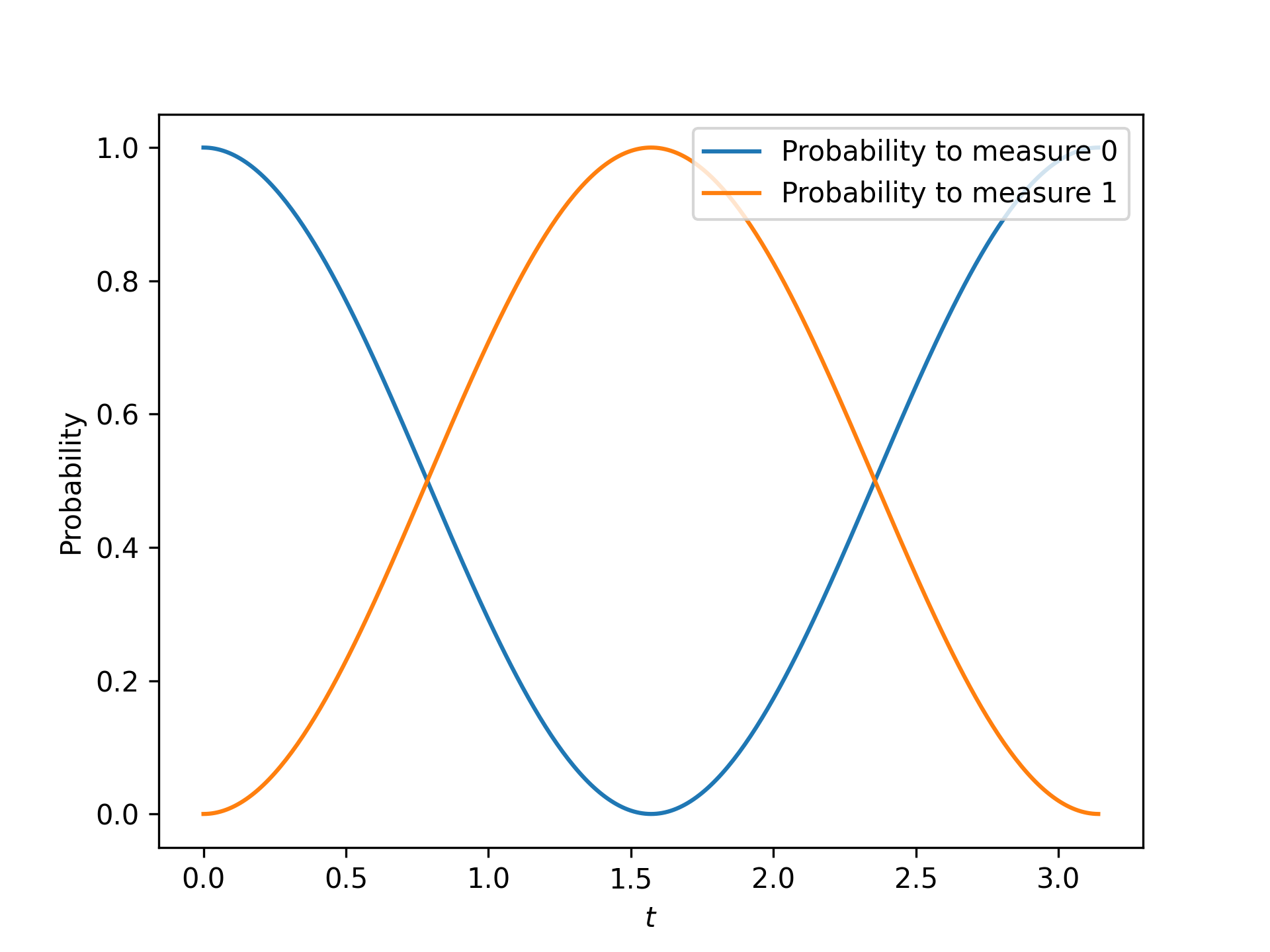
Probabilities of measuring 0 and 1 when the state \(\ket{0}\) is evolved by \(e^{-iXt}\) for various values of \(t\). The important Unitair concept is that we performed evolution by starting with a batch of operators \(\left(e^{-iX \cdot 0}, e^{-iX \delta t}, \ldots \right)\) and we applied the batch to the initial state \(\ket{0}\).